
| Asset | Fleet of Jet Engines (260 Units) | |
| Dataset | Engine Unit info with 3 Operational Setting values and 21 sensors. (x260 Units) | |
| Dataset Explanation | Dataset records data for all units that are Run-to-Failure (RTF) On-board sensor values are recorded once for each flight cycle. Dataset: 260 Units Min. Cycle of an engine is 128 cycles and Max Cycle is 378. Published by NASA CMAPSS, this dataset is based on physical models simulation & validated with real data. | |
| Objective | Calculate the Remaining Useful Life (RUL) of Test dataset Units. Build RUL model from data and predict RUL for new data. Estimate RUL with Confidence Levels. |
The problem statement can be summarized in the graphic:

The system under study is an aircraft jet engine with onboard sensors. Data from the onboard sensors are averaged out over each cycle and recorded as one-row entries. It is repeated until that Unit fails due to HPC Degradation. Each Unit from the fleet has the same sensor values recorded.

The 3 Tags: Setting 1, Setting 2, and Setting 3 has values to denote the 6 different use cases for the same Engine type. Meaning, the operating conditions are grouped into 6 clusters.
We use the historical trend data to establish a model for this Engine’s Remaining Useful Life (RUL). RUL predicts the number of cycles left in the engine before a failure. This is analogous to the Reliability (%) metric used in Asset Management.
2. Data Pre-Processing:
The given dataset is first partitioned into Training & Test Dataset. As per the split method, out of the 260 Units we have data for, 208 are split as Training data and the remaining as Test data.

Visualizing the data is the first method to employ to identify if the data is communicating any clear trends that we can use for RUL analysis. Just looking at the multiple plots below we can identify the 6 different operating conditions in the data as 6 separate clusters in each subplot.

Taking a closer look at one of the Sensor readings: HPCOutletTemp shows that the 6 clusters are clearly demarcated and that there is no trend in the pattern of sensor value for each cluster. i.e. the values tend to be flat without any increasing or decreasing trend.

Zooming into one cluster to see if there are any detectable trends. In this next investigative step, the data is also normalized to have the same range between all the sensors. We group the dataset based on the 6 operating conditions. Then the sensor reading for one operating condition is plotted. The same sensor (HPCOutletTemp) is plotted for one operating cluster below and this shows a visible trend!

All sensor readings are reviewed again by individual clusters to observe trends. Trends can be increasing or decreasing. Out of the 21 sensors, we choose the ones that exhibit Trends and combine them into one trend parameter.
3. Health Indicator
“Health Indicator” is a parameter that completely captures the behavior of the Unit. It’s also been referred to as the “Condition Parameter” or ‘Resistance to Failure”. There are numerous Feature Engineering ways to get this health indicator value from the given dataset. From the above section, we identify the top 10 sensors that have high Trendability measures.

The chosen 10 sensors are then fit to the data by assuming a Linear Degradation Equation. The condition of the system is assumed to be Linearly degrading time, which may or may not be true. There are alternate ways to fit the data into a model such as Exponential or Polynomial Degradation. Reserving those for future studies.
Now, the 10 sensors are fitted to a linear equation with 10 unknown equation parameters. Since we know the complete dataset the 10 unknown parameters are calculated. The resulting equation with 10 known equation parameter and the sensor values give us the Health Indicator. Mathematically,
y =( x1*a1) + (x2*a2) +…+(x10*a10),
where y is health indicator; x1,x2,…,x10 are sensor readings; a1,a2,…,a10 are model parameters.
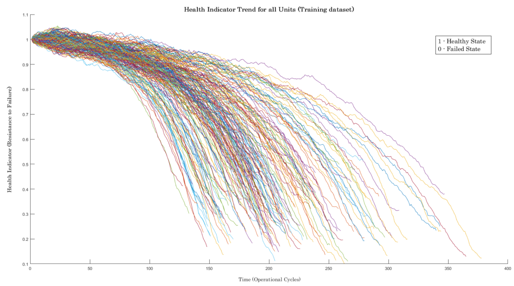
Above equation gives the health Indicator for the Training dataset. Its value is set between 1 and 0, with 1 indicating a “Healthy state” and 0 denoting the “Failed state”. The unknown parameters calculated are all from the Training dataset.
To evaluate the health indicator model, we apply the same equation to the Test dataset.

4. Building RUL Model
With the Health Indicator identified, we can build an RUL model for it. The RUL model is different from the above in that it predicts the total remaining time to reach a Health Indicator value of “0” from its current state. RUL model also looks at all the degradation trends from the above section and considers the probability of the new trend being part of that population. In other words, the degradation model is for one trend line and the RUL model is for all the trend lines combined.
For the Run-to-Failure dataset with identified Degradation pattern, we use the Residual Similarity RUL model.^ The model predicts the Estimated Remaining Useful Life and Confidence Bounds on its estimation.
We evaluate the RUL model by running it on one of the Test data readings. It will start predicting as soon as the reading start trending. For example: consider the Test data Unit#34. It ran for 179 cycles before failure occurred. If we ran the RUL model on Unit#34 at the 90th cycle, will it predict the RUL accurately?
5. Reliability Engineering
Reliability Engineers analyze data to estimate the probability of failure of an asset. RUL model gives this information in a dynamic way that keeps updating as new data is coming in. Let’s answer the question posed in the above section: at the 90th cycle for Unit#34, the trend of the Health Indicator (from the trend of the 21 sensors on Unit #34) is the red solid line. All the blue solid lines are dataset readings that are considered historical data.
RUL model takes the red solid line and predicts the RUL of 105.46 cycles within the CI band of 72.17 and 158.33 cycles. Note this is “Remaining” life, so in the plot “Est RUL”, it is at, (current cycle + predicted RUL) = (90 +105.46) = 195.46. Even though Est RUL is predicted, the Actual RUL can take a range of possible values as indicated by the shaded region pdf near the bottom of the plot. From this, we can say the probability that RUL will be at a certain value.

Continuing the analysis by re-running the RUL model for Unit#34 at Cycle 125 yields the following result. The confidence levels have narrowed as the model has had more data.
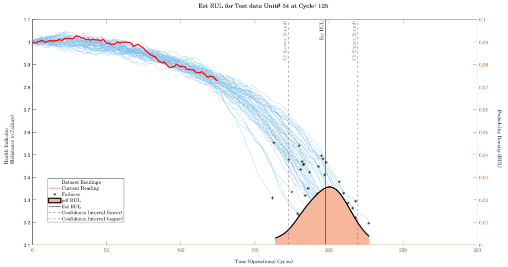
If the prediction is made at Cycle: 161 then the confidence bounds are narrower still. The prediction range narrows as more data is processed (or as cycles increases). This explains why the Prediction Error at the beginning of the Unit Life is high. It reduces as operational cycles get accumulated.

The RUL model can be applied to all the Units in the Test dataset and its respective RUL can be estimated. These predictions are with CI bounds which are not shown here.

What can Reliability & Maintenance professionals do with this result? The above model gives them the information of when this particular Unit is going to fail. Now it is imperative that the team act on this information with a judgment of whether to do a maintenance intervention. In practice, that decision is not straightforward as it needs to consider other affecting factors. The above RUL prediction shall be combined with the known MTTRs to plan & schedule. The consequences of the failure in terms of lost Uptime & Cost should also be considered.
Future Work:
- Optimize the model chosen for degradation & RUL prediction
- Include Maintenance Data in the analysis
References:
- Mathworks: Predictive Maintenance Toolbox Documentation
- NASA PCoE
- User’s Guide for the Commercial Modular Aero-Propulsion System Simulation (C-MAPSS)
Related Posts

Demo C.3: Predicting Battery Life from health data
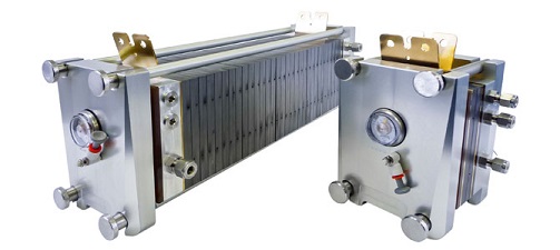
Demo A.3: Analysis of a Fuel Cell System