
| Asset | Fuel Cell stack on a test bed | |
| Dataset | 1. Ageing Data: Time, Voltage (U_Tot), Current(I), Current Density(J), Operating Sensors (18 values) 2. Polarization Data: Voltage (U_Tot), Current(I), Current Density(J) | |
| Dataset Explanation | Fuel Cell was operated on a test bed in steady state (constant current) condition and degradation were monitored. Dataset from ‘IEEE PHM ’14 Data Challenge’. | |
| Objective | Find the State of Health of the system and build an RUL model |
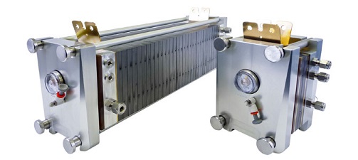
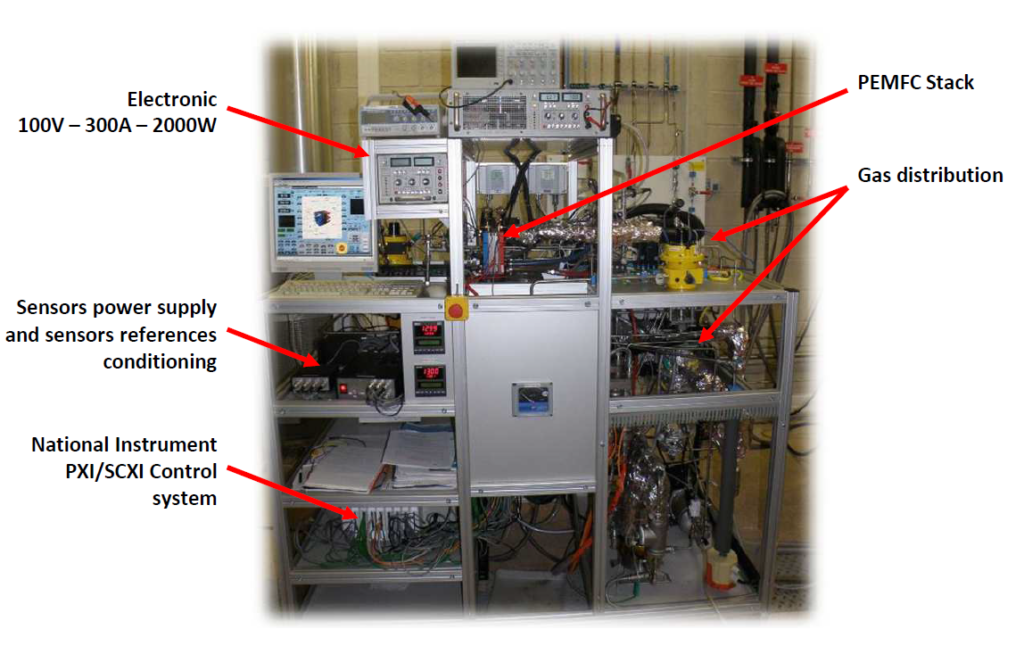
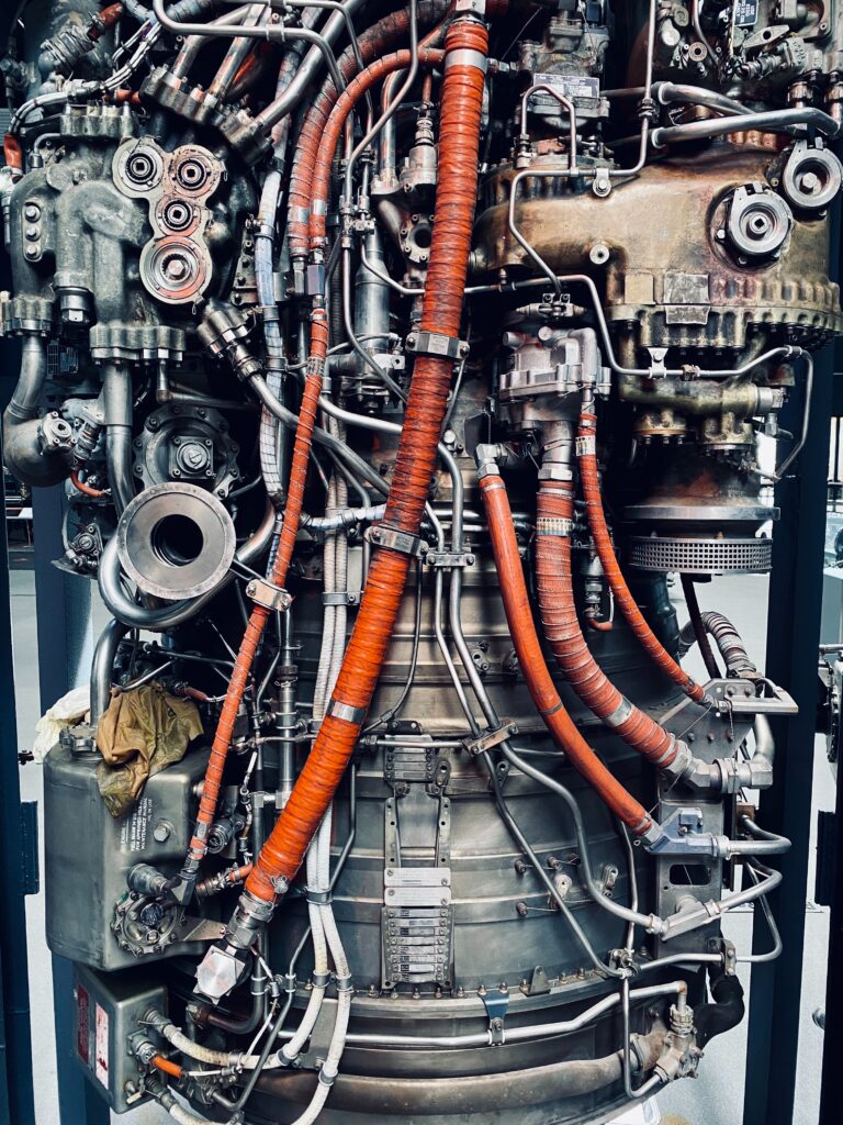
The experimental setup consists of a Fuel Cell built with 5 PEMFC cell stacks, each with an area of 100 sq cm. The nominal current density is 0.70 A/sq.cm. Fuel Cell is supported by a cooling system, fuel flow system, and controls as shown below.
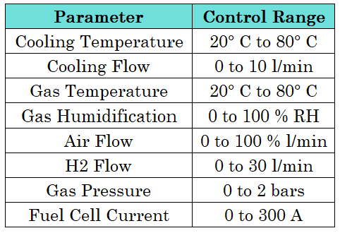
Operating parameters such as cooling temperature, airflow, and fuel flow are all controlled as per the planned experiment. The entire setup is explained in the project description document. The table of parameters for reference is:
The complete data set published has two conditions: Fuel Cell operation at Steady State and Fuel Cell operation at a Dynamic State. For the analysis here, I’m considering only the dataset under steady-state operations, i.e. without any current ripples. I’ll explore the dynamic operation dataset later in a separate blog post.
1. Data Visualization
Ageing data for the steady-state operation is a time-series syntax with operating parameter values. The stack degraded over time and the objective is to model this degradation. Before we start degradation, let’s visualize all the sensors to detect any trendability or prognosability. Ageing data in different files are collected into a single table.
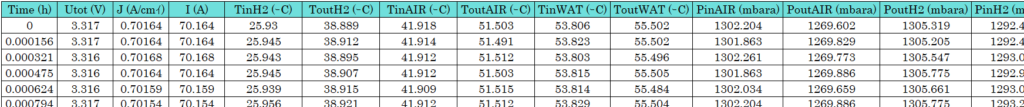
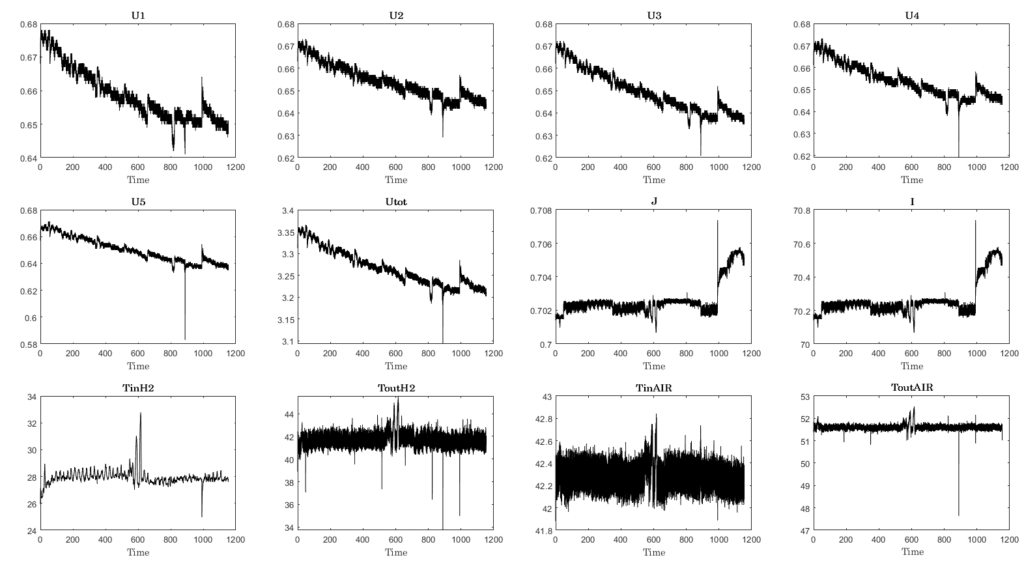
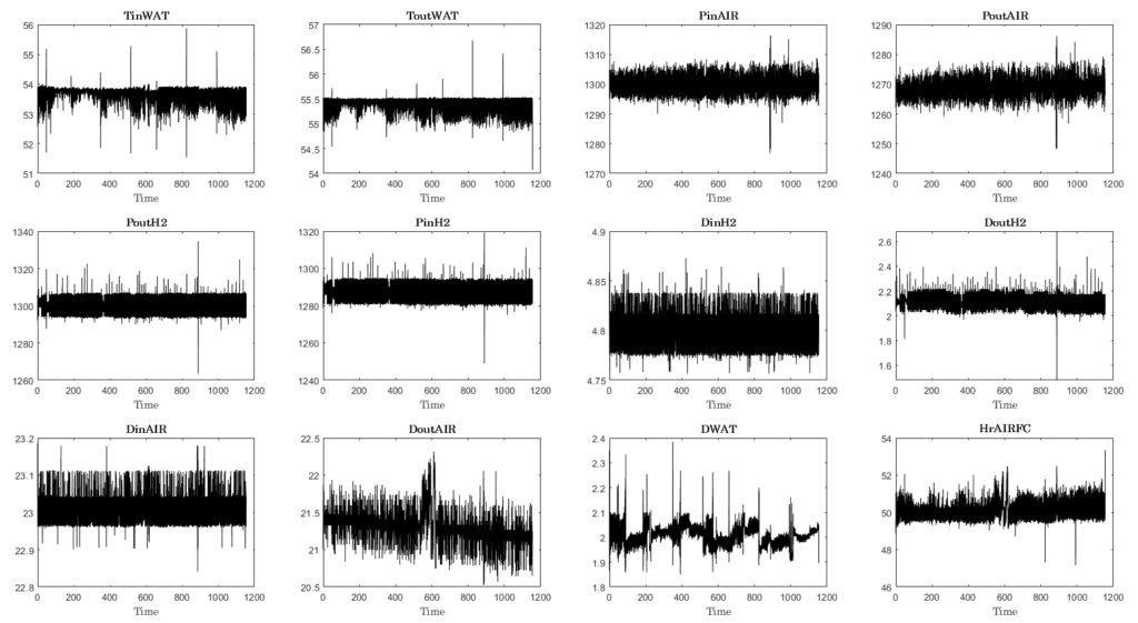
The trend of sensors is mostly constant throughout its runtime with values fluctuation around a mean. These are the operating condition sensors and they are designed to control the system within the specified range. Data from these sensors will not be useful in detecting degrdation or any failure in the fuiel cell, so we can ignore them for our analysis.
2. Data Preprocessing
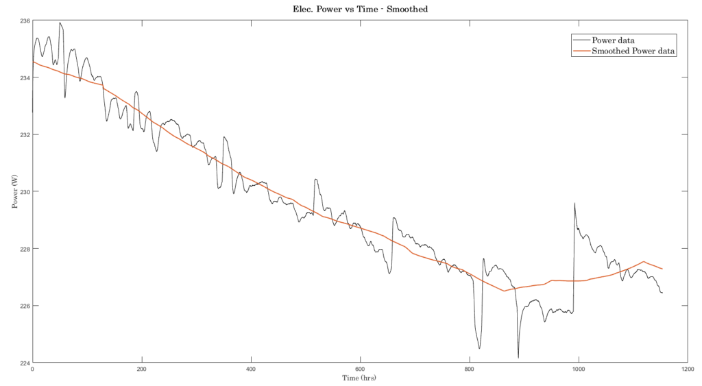
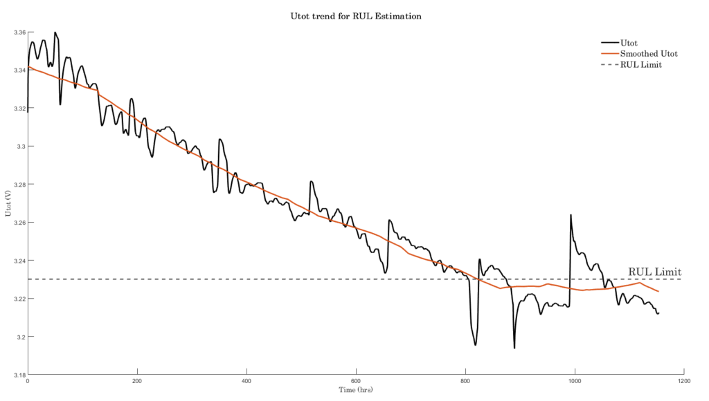
Of the sensors, a discernible trend is observed only for the Total Voltage Output for the Fuel Cell (U_tot), which is decreasing with time. Even though the general trend is downwards for Utot, it has fluctuations at points.
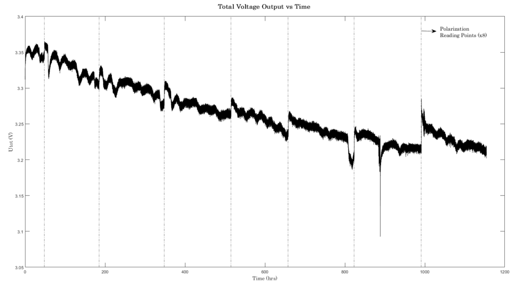
This can be explined by the times the Fuel Cell was subjected to characterization recordings. i.e. using Electrochemical Impedence Spectroscpy(EIS) to record voltage across cells to plot Polarization Curves. It was done, as per test setup desription, at times t = 0, 48, 185, 348, 515, 658, 823, 991 hrs. The spikes in data correspond to these times.
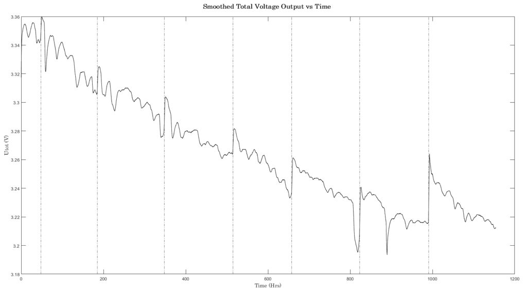
Utot data is very noisy because the readings are collected 3000 times per hours. Since the plot has Time (hours) in X-axis. We reduce the noise by taking a moving mean of the data. This smoothes the data and removes outliers.
3. Feature Selection
Above section completes preprocessing steps. Is total voltage the only parameter that we can use as Health Indicator? Literature review shows that for Fuel Cell performance monitoring, Electrical Power and Cumulative Energy might also be a good candidates for Health Indicators. Generating these two parameters from the given dataset:
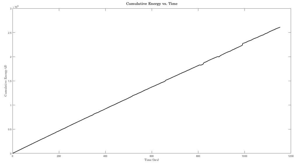
Total Voltage Output (Utot), Power (W), and Cumulative Energy (J) are all monotonic in its trend for this data. We can establish a threshold and classify the performance as degraded (Normal/Warning/Alarm).
4. Health Indicator
Having a set threshold to monitor performance degradation will work only for this specific case as the operating condition is steady state and the threshold is set for this system. If the operating conditions or the fuel cell make up change, then the threshold needs to be changed. To develop a robust method of settign up threshold, we use the Cumulative Energy produced by the cell and compare it against the Theoretical Cumulative Energy possible when there is no degradation. If the residual between these two values are greater than “set limit” then it’s an Alarm.
To calculative the Theoretical Cumulative Energy, we use the Polarization readings. The data for polatization readings are given in the dataset.
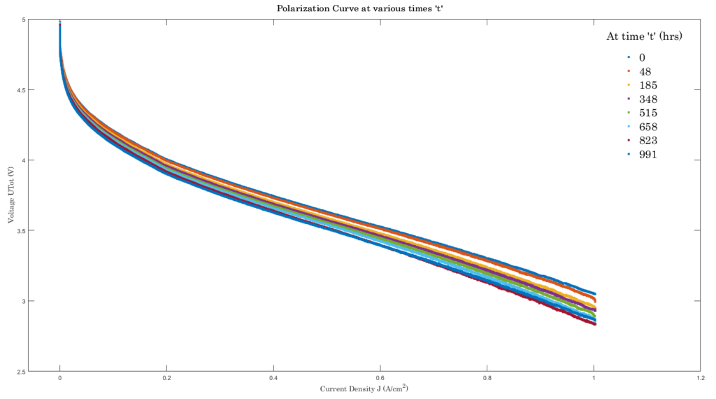
As evident from the polarization readings at various times, the voltage degrades as operating time increases. We can use the trend of the polarization curves at various times to track the performacne degradation at times. For our specific need, we use the polarization curvea t time t=0 hrs. If this behaviour is set for all the life, then it means that there is no degradation of performance. This would make a good reference curve to compare the Actual Cumualtive Energy curve against.
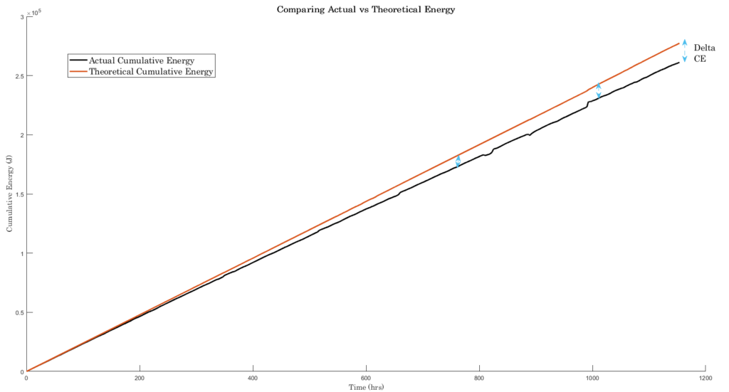
So, plotting the Actual Cumulative Energy and the Theoretical Cumulative Energy:
5. Reliability Engineering
For Reliability Engineers monitoring a Fuel Cell system like the one in test, we can look at the trend of the Delta of Cumulative Energy (Theoretical Cumulative Energy – Actual Cumulative Energy). Establish thresholds to the % of difference between these values. If we set 4% as Warning limit and 5% as Alarm limt, then we can implement a realistic PHM system.
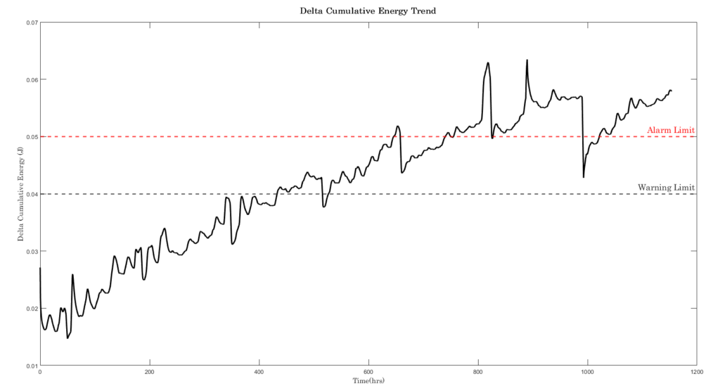
Since the dataset did not label if a failure had occurred, we are sticking to naming the thresholds as Warning & Alarm. When failure data is captured, we can then specify the limit as “Functional Failure”, and with this set we can arbitrarily locate the “Potential Failure” point to trigger alarms for the maintenance crew.
With this set up we can detect Anomalies in the Fuel Cell trend. When a fleet of fuel cells are monitored, then Anomalies can be ranked and maintenance actions be prioritized.
6. Reliability Engineering II
The second objective of our ananlysis is to estimate the Remaining Useful Life (RUL) of the fuel cell. The method to do this is by taking the most appropriate Health Indicator and fit it to a model and extrapolate to the established failure limit. Since we have only one fuel cell in our data, we can use its Total Voltage output (Utot) as parameter and fit a Linear Degradation model to it. This is one of the ways to estimate RUL. Literature has many other ways to estimate RUL such as LSTM, Exponential, etc. Chocie of RUL model comes down to practitioner. So, if we set limits for RUle stimation on linearly degrading Utot:
We can then estimate the RUL at various time points. Estimating RUL at time 400, 500, 600, 700 hrs yields the following results with Confidence Interval (upper and lower bounds).
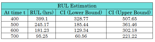
As time increases, the RUL reduces and also the CI interval shrinks as the model has got more data to make a prediction. With these predictions, Reliability & Maintenance professionals can plan the operations of the Fuel Cell System.
References:
- IEEE PHM 2014 Data Challenge
- Estimating the end-of-life of PEM fuel cells: Guidelines and metrics: https://doi.org/10.1016/j.apenergy.2016.05.076
- A Short-Term and Long-Term Prognostic Method for PEM Fuel Cells Based on Gaussian Process Regression: https://doi.org/10.3390/en15134844
Related Posts

Demo C.3: Predicting Battery Life from health data
Demo C.2: Predicting RUL of Fleet Units