Understanding Anomaly Detection (AD) with the P-F Curve

In the previous article, P-F Curve was used to understand the Remaining useful life (RUL) of an asset. RUL can be estimated at any time during the asset’s life, but it’s opportune to calculate RUL at the time ‘t’ when the asset shows signs of an impending failure. In the P-F Curve terminology the point at which the asset shows signs of failure is called the Potential Failure Point (Pf), which can also be stated as the time of anomalous behavior. The exercise of detecting anomalous behavior is called “Anomaly Detection (AD)”.

Let’s show these terms on the P-F Curve. 

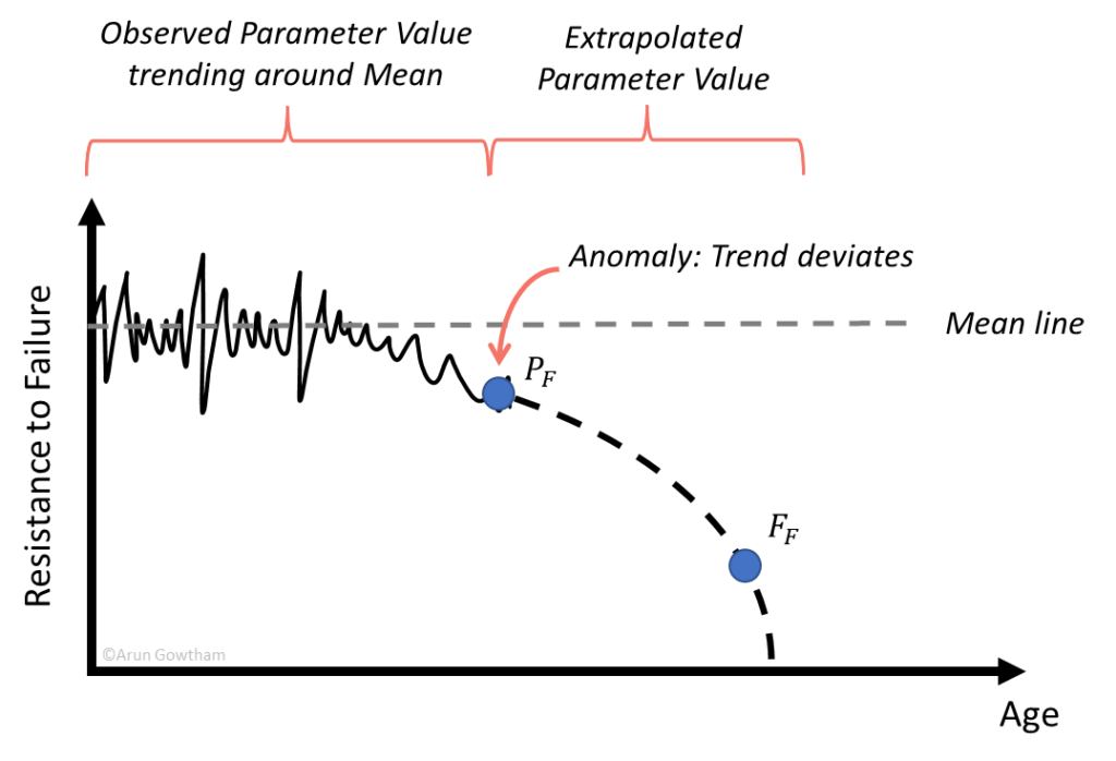
Anomaly Detection

The change in the trend of the curve is an indication of a change in the asset’s behavior, defined as an ‘Anomaly’. Maintenance practitioners who are responsible for ensuring the condition of the asset will use this anomaly detection as a notification that a repair or rework is needed to restore the asset’s functions. 

Considering all the administrative steps maintenance personnel must go through to repair an asset, it’s better to receive an alert as early as possible. Given this temptation, can we flag an asset as an ‘Anomaly’ once it reached any change in trend? 

No. The change in slope might be due to process variations or changes in operating conditions. It’s appropriate to establish a threshold limit that shows a clear deviation from the expected behavior. Limits are set from inputs such as historical performance, detection technology used, failure mechanism observed, and operating conditions. Having this limit established and agreed upon will increase the efficacy of detecting True Anomalies rather than False Positives. The threshold Limit on the P-F Curve will look this: 

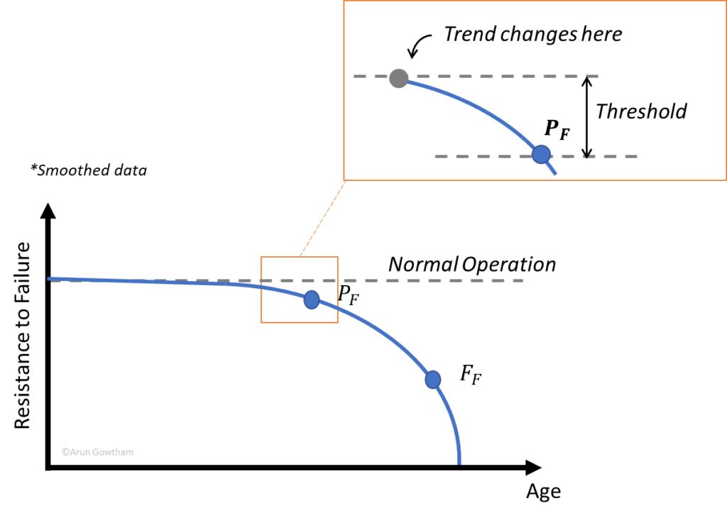
Thus, we can update the definition of an ‘Anomaly’ as follows:

Anomaly is the point at which the asset’s behavior deviates more than the threshold established for the same operating conditions”

If the operating conditions change, then the threshold limits should change too. For example: having a vibration anomaly alert limit at 0.04 in/s on a vehicle engine is good for operations on city roads but if the user drives the vehicle off-road traversing rocky terrain, then the limits should be higher. 

Setting Limits

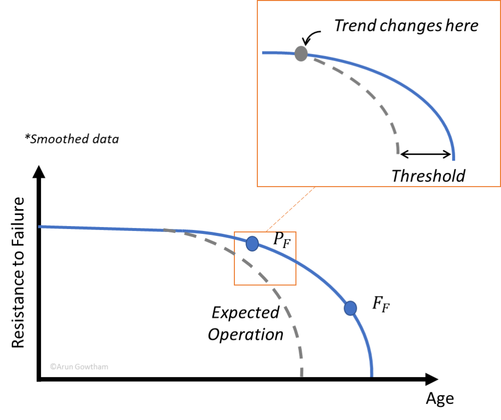
Setting up threshold limits is not reserved only for the initial degradation detection; it can also be used to compare the rate of ‘actual’ degradation against ‘expected’ degradation. For instance, if you know how your asset’s performance will degrade over time then you can set that expected rate as the baseline threshold and calculate the current rate’s deviation from it. This is represented in the figure on right. 

Another thing to consider is the number of points trending beyond the threshold limit. Is it an Alarm if the trend breaches the threshold limit only once and gets back? Or what if it alternates above and below the threshold line? How do we determine an alarm? The answer depends on the failure mechanism and Severity.

Cumulative Limits

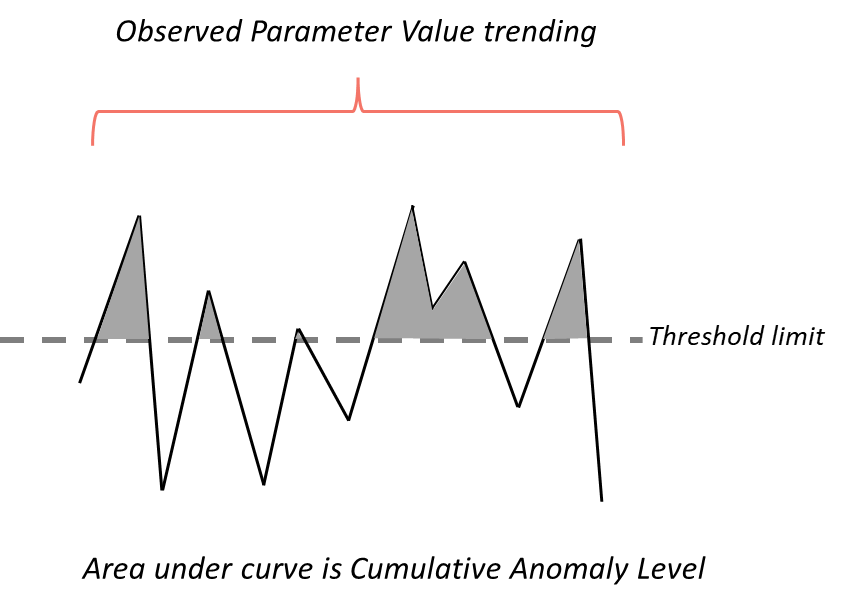
Fatigue, Thermal cycles, or any failure mechanism that follows the S-N curve needs to consider the accumulation of stress. For these, look for the cumulative breach value. The area under the curve of all the limit breaches gives you the Cumulative Anomaly Score. Depending on the magnitude, an alarm can be raised immediately or only after the Cumulative Anomaly value is higher than a defined value. 

Use this understanding to find how the software or digital application in your organization is determining an Anomaly alert. A pre-packaged threshold limit given by the software might not apply to your operation.